Full Signal Analyses: The Next Step in Biomechanical Analysis

Over the past two summers, our biomechanics lab has become the driving force behind our athlete training and development programs. We just finished the second summer, and are consistently impressed with the quality of the reports. Using these reports, we can pinpoint an athlete’s specific mechanical deficiencies, and then address them via targeted drills and exercises.  We’ve looked at that a little bit in a previous blog post. You can check out a sample biomechanics report here and see how you can look at biomechanics with the software Mokka.

While biomechanics reports have been very effective in helping us identify and resolve mechanical issues, they are limited in that they only display measurements at specific times: torso flexion at ball release, elbow extension at foot plant, maximum shoulder IR speed, etc. Sure, it’s helpful to look at metrics at key events like foot plant and ball release, but what happens in between? 

Think about it like comparing still pictures to video. 

See how much information you’re potentially missing in between? 

Instead of comparing two athletes’ elbow flexion at the events of foot plant, max external rotation, and ball release, what if we compare their elbow flexion through the entire delivery? This is what we mean when we talk about full signal analysis—analyzing every data point in time for each person’s delivery. Instead of choosing a handful of points at key events, we look at all of the data points at all possible events. 

Intuitively, it seems like we’re discarding a lot of data by collecting at 240 Hz, only to pick out discrete points for statistical analysis. 

Full signal analyses are becoming more popular in clinical biomechanics, but they are scarcely used in the baseball world. We aim to fill that gap.

Methods

In order to compare full signals, we used something called a statistical parametric mapping (SPM) technique. This technique is used to treat continuous functions of time, rather than discrete points. Statistical tests are performed on every single data point, rather than at a single one. Think of it like a t-test over time, rather than for a single point. 

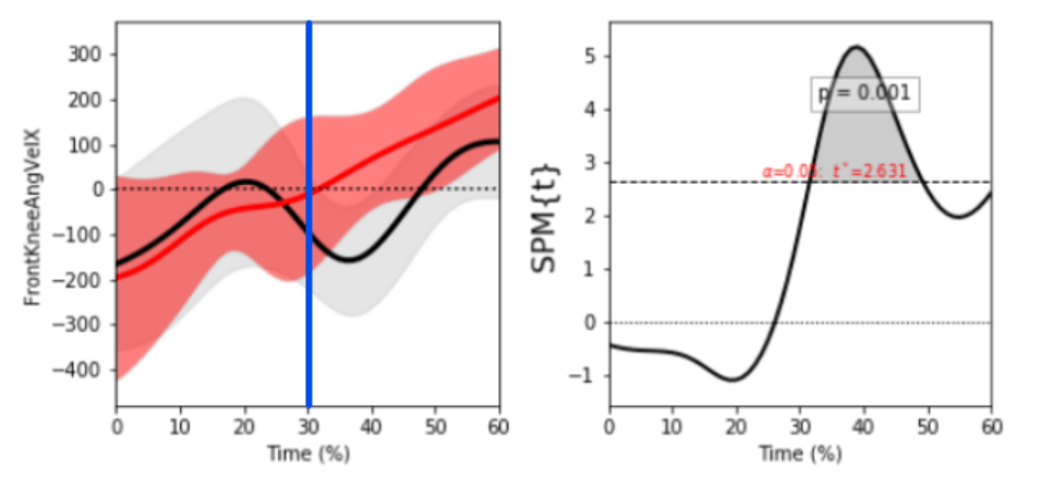
Here is what a sample SPM analysis looks like: 

The graph on the left shows the two signals that are being analyzed. The graph on the right is a measure of statistical difference at each point in time. If that value is close to zero, the graphs are not significantly different. If that value is higher than the t’ value, then the signals are significantly different, as indicated when the area under the curve is shaded.

In order to perform an SPM analysis, signals must be normalized to the same length. Every pitcher takes a different amount of time to deliver the ball to the plate, so these times must be adjusted to allow comparison. One athlete might take 1 second to deliver the ball (or 240 frames), whereas another might take 1.25 seconds (or 300 frames). These signals must all be normalized to the same number of data points. For our analysis, we normalized the signal from peak lead-leg lift until ball release as 300 frames. 

We then split our data into two groups based on velocity bins. We looked at athletes who threw above 88 mph in motion capture (n=14) and those who threw below 76 mph (n=25). We zoomed in on the area around footplant, with a window of 30 normalized frames on either side, and performed an SPM test.

Results

After running the analysis, we found that four different relevant metrics were significantly different between the hard-throwing group and the soft-throwing group.

In all of the graphs below, 0% is 30 frames before foot plant and 60% is 30 frames after foot plant. The blue line is foot plant. Hard-throwers are represented by the red line, soft-throwers by the black.

Pelvis Angle:

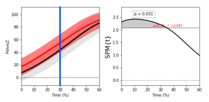
Pelvis angle is defined as the angle of the pelvis relative to home plate. 90 degrees would be facing towards home plate, 0 degrees would be facing towards third base for a righty, or towards first base for a lefty.

Looking at the graph on the left, we can see clear differences between the red and black lines. The graph on the right shows where the signal is significantly different. So, we can see on the right graph that pelvis angle is significantly different before foot plant and just after foot plant in harder throwers, but not significantly different later after foot plant.

This means that harder throwers have a more “open” pelvis as they move into foot plant compared to slower throwers. 

Pelvis Angular Velocity:

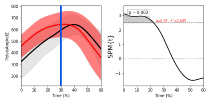
Looking at pelvis angular velocity (how fast the pelvis rotates), we see a similar pattern to the one displayed in the pelvis angle graphs. The curves are significantly different before foot plant, with harder throwers reaching their top pelvis angular velocity before the slower throwers. 

Note that the harder throwers aren’t necessarily rotating their pelvis at a faster velocity; the rotation just occurs sooner in the delivery.

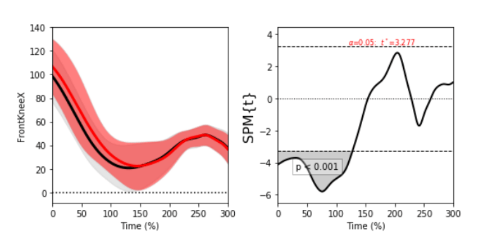
Lead-Knee Extension Angular Velocity:

Lead-knee extension angular velocity—the speed at which the front knee extends—is one of the metrics we use to quantify the “lead leg block”, which has been shown to be significantly correlated with ball velocity. 

Here we see that the difference between harder and softer throwers is most significant just after foot plant. Right at foot plant, the harder throwers (red line) are very close to 0 deg/s extension velocity, and are trending positively. The softer throwers (black line) are significantly negative and trending even more negatively, until they finally start to actually positively extend their knee.

What does this mean? It means that the harder throwers are beginning to extend their knee and block as soon as their front foot hits the ground. The soft throwers, on the other hand, sink into their lead leg and start extending much later—indicating a weaker lead-leg block.  

This difference is visible in harder throwers whose front knee doesn’t sink at all at foot plant and immediately begins extending (positive velocity), compared to slower throwers who sink further into front knee flexion (negative velocity). 

In the pitching motion of elite throwers, the window of time to transfer momentum is very small, so a pitcher needs significant impact force to achieve the imMotus needed to change momentum. Slower throwers on the other hand will plant and then sink further into foot plant, transferring their momentum too late in the throw, which causes them to miss out on efficient kinematic sequencing. 

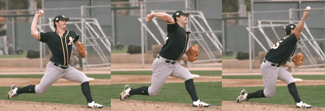
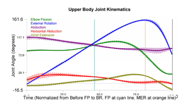
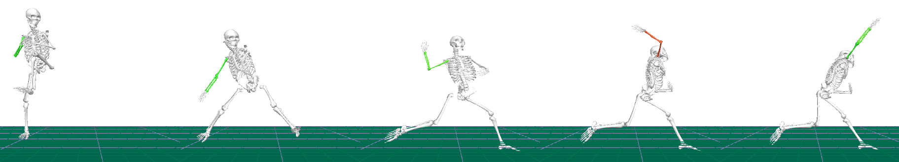
Here’s a great example of immediate lead-knee extension following foot plant from a 90+ mph arm during their motion capture assessment in the gym:

Notice that the knee angular velocity (bottom graph) is positive through the whole block

COG Velocity:

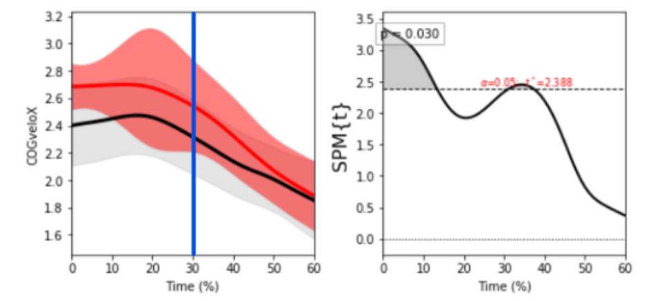
COG Velocity is the speed at which the pitcher’s center of gravity moves towards home plate. Here we see that before foot plant the harder throwers are moving significantly faster than the slower throwers. 

What is interesting is that despite moving significantly faster down the mound, the harder throwers still have better lead-leg blocks. The harder throwers are not only able to generate more momentum towards home plate, but are also able to block that greater amount of momentum more quickly and efficiently after foot plant. 

How? Strength likely plays a large role, but it’s likely that that other kinematic positions play into it as well. It’s possible that due to the pelvis rotating earlier and being more open at foot plant,the lead leg can be in a more efficient position to extend and block all of that momentum. It could also be a variety of other factors that we don’t know about yet. 

Wrapping Up

It shouldn’t be surprising that in order to deliver a baseball at elite velocities, a lot of things have to go right at the right times. Traditional biomechanical analyses have looked at kinematic metrics at certain points in time, but those only give you a snapshot of what’s happening throughout the entire course of the throw. SPM and full signal analysis give us the full picture, and can tell us what matters at any point during the throw—not just at key events. 

Which would you rather use to analyze pitching mechanics, this:

Or this? 

There’s still a lot that we don’t know about pitching mechanics and how the world’s best can throw at such extreme speeds. Improvements to our lab, like adding force plates, as well as deeper investigations like SPM and computed muscle control will only continue to help us learn more about pitching and enable us to develop better programs to train our athletes. These types of analyses are what put Driveline at the forefront of pitching research and development. 

This article was written by:

Alex Caravan, Quantitative Analyst

Anthony Brady, Lead Biomechanist

Kyle Lindley, Biomechanist

Joe Marsh, Director of R&D