Sample Sizes at the Major League Level

I’m obsessed with sample sizes. And I think anyone looking to draw any sort of conclusions off data should be.

The world of analytics has come far in recent years, but the critical area of research that deals with reliability in drawing conclusions off certain sample sizes has still left a lot to be desired. Specifically, anyone interested in the projectable nature of sample statistics should be deeply interested in what the benchmark for the appropriate n, or number of data points in the sample, to reliably project the number as a stable indicator.

That’s not say there hasn’t been some research: Pemstein and Dolinar have helped raise the bar high and set out an intuitive approach to sample size, in their (in my eyes) instrumental piece here and they reference even earlier work done in much the same vein by others like Russell Carleton, while Adam Dorhauer provided a few applicable situations for putting the gory math to work.

Warning: There are a few technical, math details below, which aren’t instrumental to the broad understanding of this piece but are included for replicability purposes and the the mathematically curious.

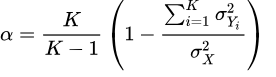
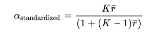
However, almost all past research has stayed at largely plate-appearance level (or the even more infrequent event of a BIP, or Ball-In-Play) and used only Cronbach’s alpha as a measuring device, which is the average of all split-half reliability coefficients, stemming from splitting each sample size in half and measuring correlations. Below, you also find the equations for the raw Cronbach’s alpha on the left and the standardized Cronbach’s alpha on the right.

A delineation of the variables included:

• K denotes the number of individual samples, 
•  denotes the variance between the samples,
•  denotes the variance of pitches among all samples,
• and  denotes the mean of the [K * (K-1)] / 2 number of non-redundant correlation matrix values.

As mentioned above, many of the findings have revolved around finding the appropriate sample size for plate-appearance metrics, like walks, strikeouts, home runs, etc. In this piece, however, we examined the following pitch-level metrics (taken from separate player seasons between 2008 and 2017):

1. Zone Swing %
2. O-Zone Swing %
3. Contact %
4. SwStrk%

We also employed an assortment of different methodologies to validate our findings below.

Although not totally clear, it seems from the explanation given in previous research that the “raw” covariance-based Cronbach’s alpha was used as a measure of score, which is often sensitive to differences in row variances, where the rows are going to be player-specific sequences of pitch-specific column values. We instead decided to go with the standardized alpha, which is based on the correlations between samples. The rationale being that pitch samples with additional variance will be given extra weight if the individual items (or rows of data) are not standardized. Given that we have a congeneric model where each line of the matrix (Xi = bi*T + Ei) and each item doesn’t measure the “true talent level” of individuals (as these numbers are to an extent dependent on opposing pitcher, ballpark, umpire strike zone, etc) but some items are more highly correlated with the “true talent level,” the raw and standardized alpha are not equal. (They would be if a parallel tests model held, where each item is measuring the same underlying talent level and the error items are equal.) If desired, a more in-depth discussion on the use of raw vs standardized alpha is available.

An example of what the first 5 rows of a covariance matrix would look like for a 10-pitch sized sample follows:.

cov(X,Y) X	Pitch_1	Pitch_2	Pitch_3	Pitch_4	Pitch_5	Pitch_6	Pitch_7	Pitch_8	Pitch_9	Pitch_10
Player 1	0	0	1	0	0	0	0	0	0	0
Player 2	0	0	0	0	1	0	0	0	0	0
Player 3	0	0	0	0	0	0	1	0	0	0
Player 4	0	0	0	1	0	0	0	0	0	0
Player 5	1	0	0	0	0	0	0	0	0	1

Caption: 1 denotes the presence of a “swinging strike” within each pitch; 0 denotes the lack thereof. The smallest matrix actually constructed had 40 columns and over 100,000 rows of N-sized pitch samples.

In addition, we relied not only on Cronbach’s alpha but also looked at composite reliability, which combines the true-score variances and covariances with factor loadings in a confirmatory factor analysis and does away with many of the assumptions that Cronbach’s alpha adheres to. Although composite reliability is seen as a universally superior form of loading when it comes to specific construct-factor loading, this advantage is not specifically important when evaluating the outcomes of separate baseball pitches. We still included it alongside Cronbach’s alpha in order to account for potential inequalities in error variances or measurements of correlated error amongst our player-specific list of pitches, a reported-drawback of Cronbach’s alpha. Additionally, for those interested, there is a list of more circumstance-dependent reasons to use composite reliability over Cronbach’s. Composite reliability can be mathematically described as (A)2 / [(A)2 + B ],where A represents the standardized loading for each item variable and B represents the variance from random measurement error.

To summarize, we don’t necessarily advocate composite reliability as a superior form of reliability in this situation, as factor-loading is not recommended, but we wanted to provide a possible additional benchmark in case the two measures signal different sample sizes—that in of itself would be interesting and might raise up relevant questions.

Looking at the pitch-level data from seasons 2008 through 2017 (and splitting each player season by year to account for differences in player skill or tendencies), we looked at reliability figures for a sequence of pitch numbers (from 40 to 75 pitches, which was enough in all of our main four cases to reach the general cutoff of 0.5 Cronbach’s alpha or composite reliability that was employed in previous cases).* The sequential list of pitches was first ordered by batter after each full-sized sample (which changed based on the the eight-different incremented cutoffs we ran through the data) was arranged as the rows of a covariance matrix, which was then run through a series of reliability measures. Here are the totals for the four metrics:

O-Zone Swing %
Pitches	Cronbach’s Alpha	Composite Reliability
#40	0.4461	0.4439
#45	0.4739	0.4718
#50	0.4970	0.4949
#55	0.5182	0.5143
#60	0.5370	0.5333
#65	0.5551	0.5514
#70	0.5714	0.5674
#75	0.5852	0.5814
Zone Swing %
Pitches	Cronbach’s Alpha	Composite Reliability
#40	0.3526	0.3511
#45	0.3864	0.3848
#50	0.4182	0.3848
#55	0.4434	0.4420
#60	0.4693	0.4677
#65	0.4913	0.4899
#70	0.5147	0.5137
#75	0.5311	0.5299
Contact %
Pitches	Cronbach’s Alpha	Composite Reliability
#40	0.5230	0.5190
#45	0.5491	0.5453
#50	0.5710	0.5666
#55	0.5913	0.5869
#60	0.6110	0.6071
#65	0.6276	0.6231
#70	0.6427	0.6378
#75	0.6581	0.6535
SwStrk%
Pitches	Cronbach’s Alpha	Composite Reliability
#40	0.3909	0.3909
#45	0.4159	0.4145
#50	0.4376	0.4357
#55	0.4580	0.4559
#60	0.4762	0.4742
#65	0.4956	0.4935
#70	0.5103	0.5079
#75	0.5261	0.5230

Now these calculations suggest that Cronbach’s standardized alpha and the composite reliability residual-variable calculations found themselves largely in agreement. To be clear, the suggestion here is that the sample size is large enough to expect the next similarly sized sample to replicate the same level of incidence in said metric.

• 55 pitches for a reliable O-Zone Swing %
• 70 pitches for Zone Swing %
• 40 pitches for Contact %
• 70 pitches for SwStrk %

These calculations were again calculated from over 7-million pitches thrown at the major league level over the last decade and can help us in pinpointing emerging trends of plate discipline or classifying players in buckets as soon as possible.

Of course, this is just the tip of the iceberg, a general look into any number of different permutations and combinations that arise from a sequence of pitches at the game level. (A more concentrated delve into the recent couple years where the shift to the three true outcomes could indicate different sizes of n). We just wanted to get begin looking at the reliability of progressively more discrete units. Catch us next month when we look at what happens during millisecond-intervals of pitches.

(Joking)

(Maybe)

*The 0.50 cutoff comes from the idea of accounting for the “majority” of the variance in the same setting.

References

525,600 Minutes: How Do You Measure a Player in a Year? | FanGraphs Baseball. Available at https://www.fangraphs.com/blogs/525600-minutes-how-do-you-measure-a-player-in-a-year/ (accessed July 27, 2018).

A New Way to Look at Sample Size | FanGraphs Baseball. Available at https://www.fangraphs.com/blogs/a-new-way-to-look-at-sample-size/ (accessed July 27, 2018).

Regression with Changing Talent Levels: The Effects of Variance | The Hardball Times. Available at https://www.fangraphs.com/tht/regression-with-changing-talent-levels-the-effects-of-variance/ (accessed July 27, 2018).

Falk C., Savalei V. 2011. The Relationship Between Unstandardized and Standardized Alpha, True Reliability, and the Underlying Measurement Model. Journal of personality assessment 93:445–53. DOI: 10.1080/00223891.2011.594129.

Cortina JM. 1993. What is coefficient alpha? An examination of theory and applications. Journal of Applied Psychology 78:98–104. DOI: 10.1037/0021-9010.78.1.98.